Variable Retention Times Across HPLC Runs
Practical guide to diagnose Variable Retention Times Across HPLC Runs: root causes, diagnostic checks, and fixes to stop run-to-run drift.
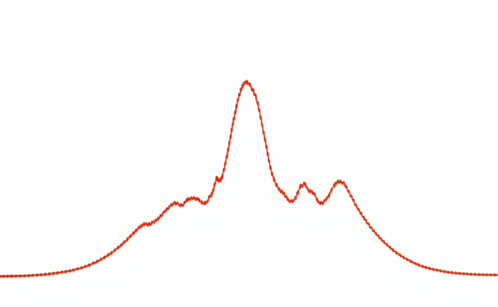
Variable retention times (tR) across high-performance liquid chromatography (HPLC) runs represent one of the most common and disruptive forms of chromatographic instability. When retention drifts, even if peak shape and resolution appear acceptable, the analytical consequences can be substantial: peak identification becomes less certain, system suitability may fail, and quantitative precision degrades. Retention time stability is not just a “nice-to-have” metric—it is a direct indicator that the mobile phase, temperature, flow delivery, gradient timing, and column environment are being reproduced run after run.
This guide explains why retention times shift, how to diagnose the dominant cause efficiently, and how to stabilize retention using practical, defensible controls. All equations are shown below as plain text (not formatted math), so they paste cleanly into rich text editors.
1) Conceptual Foundation: What Controls Retention in HPLC?
Retention in HPLC is governed by how strongly an analyte interacts with the stationary phase relative to the mobile phase. In reversed-phase HPLC, retention is largely driven by partitioning into the hydrophobic stationary phase, with additional contributions from hydrogen bonding, dipole interactions, residual silanol interactions, and (sometimes) metal or active-site effects. In other modes (HILIC, ion-exchange), ionic environment and surface interactions can dominate.
Retention time shifts occur when the effective chromatographic environment changes, even slightly. Common “silent” changes include:
A small drift in organic modifier percentage (even 0.5–1.0% absolute)
A small pH shift (especially near an analyte’s pKa)
A small temperature drift (1–2 °C is often enough to matter)
A change in gradient delay timing (dwell volume effects)
Incomplete re-equilibration between runs
Flow delivery inaccuracies (true flow differs from displayed flow)
Injection solvent mismatch (diluent stronger than initial mobile phase)
Because these variables are coupled, the most efficient troubleshooting approach is to use normalized metrics (like k) and a structured workflow that isolates composition vs. hydraulic vs. thermal vs. column/sample effects.
2) Key Definitions and Metrics (Plain-Text Equations)
Retention time (tR)
Definition: Time from injection to the peak apex.
Hold-up time (t0)
Definition: Time of an unretained marker passing through the column.
Interpretation: Reflects system volume and flow (column void + extra-column volume).
Capacity factor (k)
Plain text formula:
k = (tR − t0) / t0
Why k matters: If your tR is moving because t0 is moving (flow or volume effects), k will often reveal that quickly. Tracking k is usually more diagnostic than tracking tR alone.
Isocratic flow dependence (rule relationship)
Plain text relationship:
tR is proportional to 1 / flow
Practical meaning: if the true flow increases by 2%, tR typically decreases by ~2% in isocratic runs.
Dwell volume (Vd) and gradient delay time
Plain text formula:
gradient delay time = Vd / flow
Example (plain text):
If Vd differs by 0.5 mL and flow is 0.5 mL/min, then the gradient delay difference is:
0.5 mL / 0.5 mL/min = 1.0 min
This is why the same gradient method can “shift” by minutes when moved between instruments with different dwell volumes.
3) Why Retention Times Shift: Mechanisms with Practical Interpretation
3.1 Mobile Phase Composition and Preparation
Organic fraction is one of the highest-leverage variables in reversed-phase HPLC. Many compounds show steep changes in retention with small composition differences. This is why mobile phase preparation technique can dominate retention stability.
Key mechanisms:
Organic strength drift: Small absolute changes in %B can produce large retention shifts, especially for moderately retained analytes.
Volumetric mixing error: Measuring solvents by volume at different temperatures introduces density-related composition error. This can be enough to shift retention measurably.
Solvent lot variability: Trace impurities, water content, or additive purity can shift selectivity (not just retention time).
Degassing artifacts: Microbubbles can cause pump slip or proportioning artifacts, creating effective composition errors even if you prepared the mobile phase correctly.
CO2 absorption: CO2 dissolving into aqueous phases can lower pH in low-buffer systems, indirectly shifting retention for ionizable analytes.
Practical interpretation: If the entire chromatogram shifts earlier/later without obvious changes in peak shape, suspect composition, flow, temperature, or dwell timing first.
3.2 pH, Buffer Species, and Ionic Strength
For ionizable analytes, retention is often dominated by ionization state. A small pH change near pKa can produce a large change in the neutral/ionized fraction, and the neutral form often retains much more strongly in reversed-phase HPLC.
Plain-text Henderson–Hasselbalch forms (for context):
For an acid:
pH = pKa + log10([A−]/[HA])For a base:
pH = pKa + log10([B]/[BH+])
Practical meaning (no new numbers beyond your text): If your analytes have pKa values close to the method pH, you should expect retention time sensitivity. This is amplified when buffer capacity is low, the pH meter is not tightly calibrated, or the pH is measured at a different temperature than the method runs.
Ionic strength matters because it changes how charged species interact with the stationary phase and can reduce or enhance secondary interactions (including silanol effects), shifting both retention and peak shape.
3.3 Temperature Control and Thermal Equilibration
Retention is temperature-dependent because partitioning/adsorption equilibria depend on enthalpy. In practice, even small temperature differences between runs can move retention, especially for strongly retained analytes.
Common reasons temperature varies in real sequences:
Not waiting long enough after changing the oven setpoint
Turning the oven fan on/off mid-sequence (changes heat transfer)
Solvent entering the column significantly cooler/warmer than the oven setpoint
Inadequate preheating so the column inlet experiences a temperature transient
Practical interpretation: If retention drifts gradually through a sequence (especially early), temperature stabilization and re-equilibration time are prime suspects.
3.4 Flow Rate and Pump Performance
In isocratic mode, the relationship is straightforward:
Plain text reminder:
tR is proportional to 1 / flow
So even small flow delivery differences can become visible in retention time. In gradient mode, it gets more complex because flow differences also change gradient slope delivered to the column.
Mechanisms that create “invisible” flow and composition issues:
Check valve leakage or sluggish response
Seal wear causing flow pulsation
Proportioning inaccuracies (especially quaternary pumps)
Compressibility compensation mismatch when switching between MeOH and ACN systems
Microbubbles leading to intermittent compressibility artifacts and timing errors
Practical interpretation: If retention sometimes “jumps” instead of drifting smoothly, microbubbles, check valves, or proportioning irregularities become more likely.
3.5 Gradient Formation, Dwell Volume, and Re-Equilibration
Dwell volume differences are one of the most common causes of retention mismatches across systems, especially during method transfer.
Plain text formula:
gradient delay time = Vd / flow
If Vd differs between instruments, the gradient reaches the column earlier or later, shifting all gradient-dependent retention times.
Re-equilibration is equally critical. If the stationary phase has not returned to the initial condition before the next injection, retention will drift, often cumulatively.
This is especially pronounced in:
HILIC (water fraction and salt equilibration dominate)
Ion-exchange (counterion equilibration)
Any method with strong adsorption or slow surface equilibration
3.6 Column-Related Factors
Columns are chemical reagents as much as they are hardware. Retention changes can result from:
Batch-to-batch stationary phase variability
Differences in endcapping quality or ligand density
Column conditioning state (new columns often drift early)
Aging effects (ligand loss, pore changes, altered silanol activity)
Physical voids/bed settling (changes t0 and retention behavior)
Guard columns and frit/fitting differences can also shift early retention by changing extra-column volume and inlet dynamics.
3.7 Sample, Diluent, and Injection Effects
Injection conditions can create retention shifts without any change to the method or instrument:
If the sample diluent is stronger than the initial mobile phase, early peaks can elute earlier and with altered shape.
Larger injection volumes increase the magnitude of this effect.
Matrix components (salts, surfactants, DMSO, excipients) can change local solvent strength or compete for active sites.
Practical interpretation: If early-eluting peaks are unstable but late peaks are relatively stable, injection solvent mismatch is a common culprit.
4) Practical Diagnostics to Isolate Root Causes (Fast, High-Information Tests)
A) Track t0 and k, not just tR
Inject an unretained marker periodically.
If t0 changes, look first at flow, plumbing volume, and temperature.
If t0 is stable but tR changes, suspect composition, pH, column chemistry, or gradient timing.
B) Composition sensitivity check
Prepare mobile phase with ±1% absolute organic modifier.
Observe whether k or tR shifts strongly for a sentinel peak.
Strong response suggests composition control is the main lever.
C) pH sensitivity check
Adjust buffer by ±0.1 pH units.
If retention responds strongly, tighten pH control and ensure adequate buffer capacity.
D) Dwell volume / gradient delay check
Perform a gradient step test and compare timing to expectations.
Confirm whether the method implicitly assumes a different Vd than the instrument.
E) Flow accuracy check
Gravimetrically collect eluent over a timed interval at operating backpressure.
F) Injection solvent test
Match sample diluent to the initial mobile phase or reduce injection volume.
If retention stabilizes for early peaks, injection conditions are implicated.
5) Controls and Best Practices to Stabilize Retention
Mobile phase discipline
Prefer mixing by weight at controlled temperature.
Document solvent lot numbers and avoid unnecessary lot changes mid-study.
Use consistent filtration and degassing practices.
Minimize air exposure for mobile phases that are pH-sensitive or low in buffer capacity.
pH control discipline
Use adequate buffer capacity where compatible.
Calibrate pH meters daily and measure pH consistently at a defined temperature.
Record pH as part of the batch record so future comparisons are meaningful.
Temperature discipline
Use a column oven with stable airflow and consistent fan settings.
Allow adequate equilibration after setpoint changes (often 20–30 minutes).
Use preheating so the column inlet does not experience a thermal transient.
Instrument configuration alignment
Measure and document dwell volume on each system used for the method.
Maintain consistent tubing ID/length and mixer configuration.
If needed, adjust gradient programs to compensate for measured Vd differences.
Injection discipline
Match diluent to initial mobile phase whenever possible.
Minimize strong solvents in the diluent.
Use the smallest validated injection volume that meets sensitivity requirements.
Column management
Condition new columns with the intended mobile phase until retention stabilizes.
Track cumulative usage and replace guard columns regularly.
Treat columns as controlled consumables, not interchangeable parts.
System suitability strategy
Use reference peaks to monitor selectivity and retention stability.
Prefer acceptance criteria involving k and resolution for sentinel peaks rather than relying on raw tR alone.
6) Quantitative Rules-of-Thumb (Plain Text)
Isocratic flow:
If flow increases by 2%, tR decreases by approximately 2%.Dwell volume:
A dwell volume increase of 0.5 mL delays the gradient by:
0.5 mL / flow (mL/min) minutes
(Other rules-of-thumb in your original text remain method-dependent; keep them as guidance, then verify empirically in your system.)
7) A Rapid 60–90 Minute Diagnostic Workflow
Equilibrate and establish baseline
Equilibrate 20–30 min at set temperature and initial composition.
Inject an unretained marker and record t0.
Check flow and gradient timing
Gravimetrically verify flow.
Run a gradient step test to assess dwell volume timing.
Perform sensitivity tests
Run ±1% organic modifier test batch.
Run ±0.1 pH test batch (if analytes are ionizable).
Evaluate injection conditions
Match diluent to initial mobile phase or reduce injection volume.
Separate system vs column
If variability persists, test a second column of the same model.
Lock controls into an SOP
Standardize mobile phase preparation, pH verification, preheating/equilibration, and dwell-volume documentation.
Brief Summary
Retention time variability is almost always traceable to reproducible physical or chemical changes in the chromatographic environment. The most common high-impact drivers are small errors in organic modifier fraction, pH drift and buffer capacity limits, temperature instability, flow/proportioning inaccuracies, dwell volume mismatches in gradient methods, injection solvent strength effects, and column conditioning/aging behavior. A structured workflow using t0 and k tracking, gradient step testing, and targeted sensitivity checks allows rapid isolation of the dominant cause and supports stable, transferable HPLC methods.